Interpolation methodologies#
Inverse of the Distance - 2D#
This interpolation technique takes into account the Euclidean distance between points and stations. A residue value is calculated for every point in the region, considering the quadratic inverse of the distance between the point and all the stations.
The formula used to calculate the residue at a specific point P is as follows:
Where:
\(P = (x_{i}, y_{j})\) represents the point where the residue is calculated.
\(dist_{2D}\) is the distance between point P and station k.
\(W_{ij}\) is the sum of station weights.
\(R_{ij}\) is the residue at point P.
This technique accounts for the spatial distribution of stations and their influence on the interpolated values, providing more accurate estimates for various geographic points.
In the context of inverse distance interpolation, the degree of smoothing at a point location is influenced by the power parameter ((p)). When the power parameter is set to 0.0, a specific behavior occurs: the interpolated value at that point location becomes identical to the observation value recorded at that precise data point.
In simpler terms, when (p) is set to 0.0, there is no smoothing applied during interpolation. The interpolated value at a given location matches the observed value at the closest data point exactly. This phenomenon is often referred to as ‘zero-distance power’ because the distance to the data point is raised to the power of 0, effectively negating the influence of other data points.
Practically, setting (p) to 0.0 means that the interpolated surface will pass through each data point without any smoothing or averaging between neighboring data points. This can be beneficial when you require the interpolated surface to faithfully replicate the observed values exactly at the data points themselves. However, it’s important to be cautious as this approach may result in a surface with ‘spiky’ behavior if the observed data points contain noise or outliers.
Here an example result of the interpolation of residuals using this methodology.
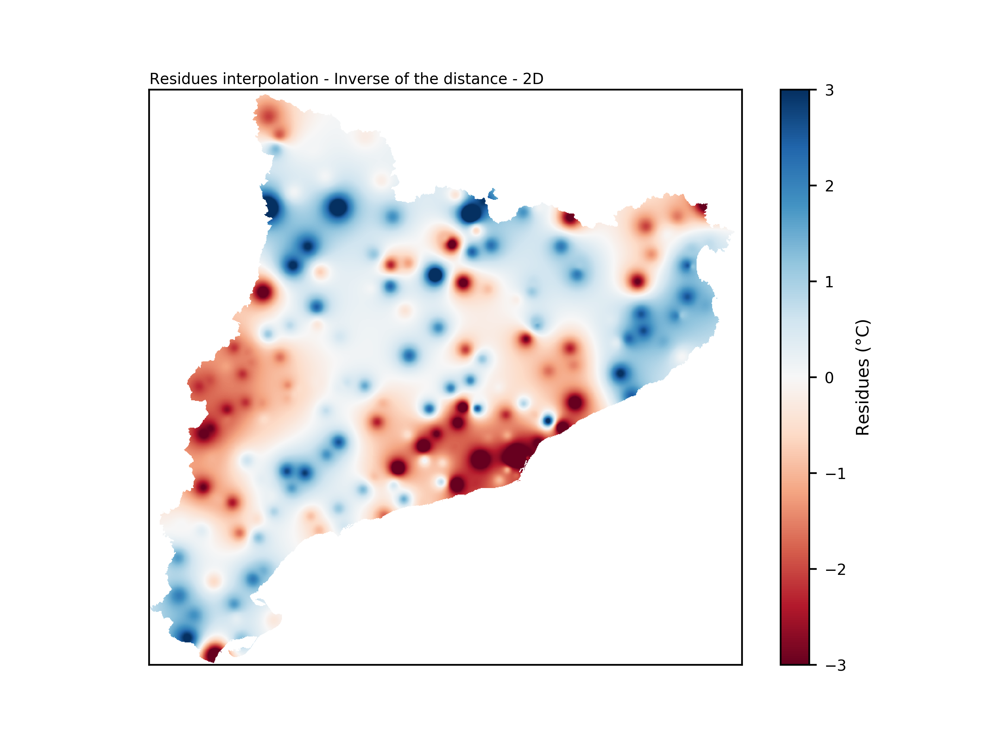
Interpolation result using Inverse of the distance - 2D.#
Inverse of the Distance - 3D#
This methodology accounts not only for the distance between a point and a station but also considers the difference in altitude. The altitude difference is multiplied by a penalization factor \(\lambda\). A higher value of \(\lambda\) results in more emphasis being placed on stations with a larger difference in altitude. In other words, if two stations are at the same horizontal distance from a point, but one station is at the same altitude while the other is 1000 meters higher, a greater distance will be associated with the second station. This methodology is adapted from Frei, 2014 and Lussana et al., 2018.
The formula used to calculate the residue at a specific point P is as follows:
Where:
\(P = (x_{i}, y_{j})\) represents the point where the residue is calculated.
\(z_{ij}\) is the altitude at point P.
\(dist_{·D}\) is the distance between point P and station k taking into account the altitude difference.
\(\lambda\) is the penalization factor for altitude difference.
\(W_{ij}\) is the sum of station weights.
\(R_{ij}\) is the residue at point P.
This methodology offers a more accurate interpolation by considering both spatial distance and altitude difference, allowing for better predictions in three-dimensional scenarios.
Here an example result of the interpolation of residuals using this methodology.
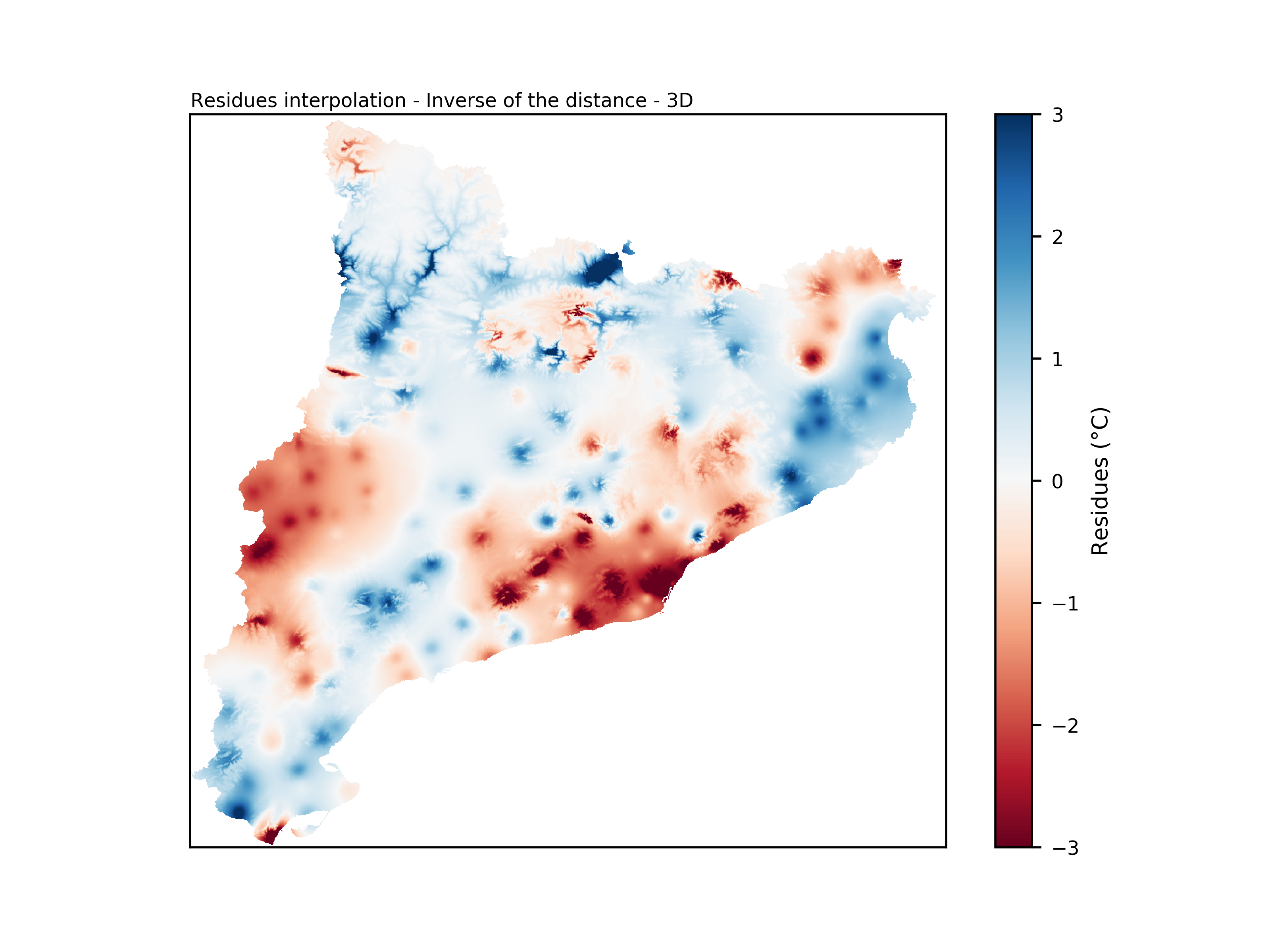
Interpolation result using Inverse of the distance - 3D.#
Multiple Linear Regression#
Multiple Linear Regression (MLR) allows for the prediction of a response variable using different explanatory variables, as opposed to only one in simple linear regressions. It can be expressed as:
Where:
\(y_{i}\) is the predictand.
\(\beta_{k}\) are the coefficients of linear regression.
\(x_{ik}\) are the predictors.
\(\epsilon_{i}\) are the residues of the regression, which represent the difference between the predicted and observed values.
In the case of MLR, the predictors are included in a forward stepwise process. First, the correlation coefficient is tested for each predictor. The one that correlates the best is selected and left out for the next step. Second, each of the remaining predictors is added to the previous regression. If the correlation coefficient combining the first predictor and the second one improves by at least a threshold of 0.05, a second predictor is considered. The one that improves the correlation coefficient the most is selected. This process is repeated until the improvement of adding one predictor is less than the established threshold or there are no more predictors available.