04. Interpolation - Inverse of the distance 3D#
In this tutorial, we’ll cover the interpolation of point data using the
inverse of the distance methodology, available in PyMica as id2d.
This methodology requires location (lon and lat), altitude
(altitude) and value to interpolate.
We’ll use Meteorological Service of Catalonia sample data to demonstrate how to apply this interpolation technique. Therefore, we need to import the required modules. First, we need to load observation data and also the PyMica class.
import json

from pymica.pymica import PyMica
Let’s call the PyMica class with the appropriate parameters, setting the
methodology to id3d and the configuration dictionary as follows:
config_file = 'sample-data/configuration_sample.json'

with open('sample-data/configuration_sample.json', 'r') as f_p:
    config = json.load(f_p)

config['id3d']
{'id_power': 2.5,
 'id_smoothing': 0.0,
 'id_penalization': 30,
 'variables_files': {'altitude': 'sample-data/explanatory/cat_dem_25831.tif'},
 'interpolation_bounds': [260000, 4488100, 530000, 4750000],
 'resolution': 270,
 'EPSG': 25831}
where:
id_power: rate at which the influence of distant data points diminishes as we move away from them.id_smoothing: if 0.0 the interpolated value at that point location becomes identical to the observation value recorded at that precise data point.id_penalization: altitude penalization factor. It influences the interpolation by taking into account the difference in altitude (elevation) between data points.variables_files: here altitude is required and the path to altitude GeoTIFF is provided.interpolation_bounds: [minimum_x_coordinate, minimum_y_coordinate, maximum_x_coordinate, maximum_y_coordinate], it must be the same as the variable files.resolution: spatial resolution.EPSG: EPSG projection code.
With all these parameters and configurations set, let’s initialize the
PyMica class with the methodology set to ‘id3d’.
id3d_method = PyMica(methodology='id3d', config=config_file)
Now that we have the interpolator set, we can input some data for interpolation. We will use data from the Meteorological Service of Catalonia AWS network.
with open('sample-data/data/smc_data.json', 'r') as f_p:
    data = json.load(f_p)

data[0]
{'id': 'C6',
 'value': 8.8,
 'lon': 0.9517200000000001,
 'lat': 41.6566,
 'altitude': 264.0,
 'dist': 0.8587308027349195}
As we can see, the first element of data meets the requirements of
PyMica input data, so we only need to call the interpolate
method from the interpolator class id3d_method.
data_field = id3d_method.interpolate(data)
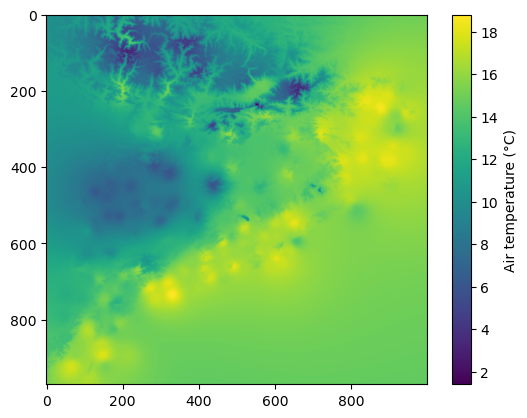
Now, we can get a quick look of the data_field array using
matplotlib.
import matplotlib.pyplot as plt

plt.imshow(data_field)
plt.colorbar(label='Air temperature (\u00b0C)')
Finally, we can save the result into a GeoTIFF file using
pymica.pymica.PyMica.save_file() from PyMica class.
id3d_method.save_file("sample-data/clusters/id3d.tif")
We have now completed this tutorial on how to interpolate station data
using the id3d methodology. You can experiment with changing the
id_penalization value to observe how this parameter affects the
interpolation result.