06. Interpolation - Multiple Linear Regression (+ residual correction)#
In this tutorial, we’ll cover the interpolation of point data using the
Multiple Linear Regression (MLR) methodology and applying a residual
correction, available in PyMica as mlr+id2d and mlr+id3d
depending on the residual correction interpolation method. This
methodology requires location (lon and lat), predictor variables
such as altitude (altitude) or distance to coast line (among
others), and value to interpolate. If mlr+id3d is selected,
altitude must be provided in the variables_files.
We’ll use Meteorological Service of Catalonia sample data to demonstrate how to apply these interpolation techniques. Therefore, we need to import the required modules. First, we need to load observation data and also the PyMica class.
import json

from pymica.pymica import PyMica
Interpolation mlr+id2d#
Let’s call the PyMica class with the appropriate parameters, setting the
methodology to mlr+id2d and the configuration dictionary as follows:
config_file = 'sample-data/configuration_sample.json'

with open('sample-data/configuration_sample.json', 'r') as f_p:
    config = json.load(f_p)

config['mlr+id2d']
{'id_power': 2.5,
 'id_smoothing': 0.0,
 'clusters': 'None',
 'variables_files': {'altitude': 'sample-data/explanatory/cat_dem_25831.tif',
  'dist': 'sample-data/explanatory/cat_distance_coast.tif'},
 'interpolation_bounds': [260000, 4488100, 530000, 4750000],
 'resolution': 270,
 'EPSG': 25831}
where:
id_power: rate at which the influence of distant data points diminishes as we move away from them.id_smoothing: if 0.0 the interpolated value at that point location becomes identical to the observation value recorded at that precise data point.clusters: set to None as no clusters will be used.variables_files: dictionary with predictor variables as keys and their corresponding GeoTIFF path as values. Here, altitude asaltitudeand distance to coast line asdist.interpolation_bounds: [minimum_x_coordinate, minimum_y_coordinate, maximum_x_coordinate, maximum_y_coordinate], it must be the same as the variable files.resolution: spatial resolution.EPSG: EPSG projection code.
With all these parameters and configurations set, let’s initialize the
PyMica class with the methodology set to ‘mlr+id2d’.
mlr_id2d_method = PyMica(methodology='mlr+id2d', config=config_file)
Now that we have the interpolator set, we can input some data for interpolation. We will use data from the Meteorological Service of Catalonia AWS network.
with open('sample-data/data/smc_data.json', 'r') as f_p:
    data = json.load(f_p)

data[0]
{'id': 'C6',
 'value': 8.8,
 'lon': 0.9517200000000001,
 'lat': 41.6566,
 'altitude': 264.0,
 'dist': 0.8587308027349195}
As we can see, the first element of the data meets the requirements of
PyMica input data and has the same predictor variables as the ones
provided in the configuration dictionary. Therefore, we only need to
call the interpolate method from the mlr_id2d_method
interpolator class.
data_field = mlr_id2d_method.interpolate(data)
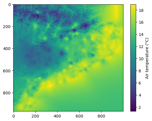
Now, we can get a quick look of the data_field array using
matplotlib.
import matplotlib.pyplot as plt

plt.imshow(data_field)
plt.colorbar(label='Air temperature (\u00b0C)')
Now, we can save the result into a GeoTIFF file using save_file()
from PyMica class.
mlr_id2d_method.save_file("sample-data/results/mlr_id2d.tif")
We have now completed the first part of this tutorial on how to
interpolate station data using the mlr+id2d methodology. The
obtained result is similar to the one in 05 Interpolation - Multiple
linear regression, but with the additional
application of residual correction, which is evident in the interpolated
field. You can experiment with changing the variables_files,
id_power, and id_smoothing parameters in the configuration
dictionary to observe how each parameter affects the interpolation
result.
mlr+id3d#
Let’s call the PyMica class with the appropriate parameters, setting the
methodology to mlr+id2d and the configuration dictionary as follows:
config_file = 'sample-data/configuration_sample.json'

with open('sample-data/configuration_sample.json', 'r') as f_p:
    config = json.load(f_p)

config['mlr+id3d']
{'id_power': 2.5,
 'id_smoothing': 0.0,
 'id_penalization': 30,
 'clusters': 'None',
 'variables_files': {'altitude': 'sample-data/explanatory/cat_dem_25831.tif',
  'dist': 'sample-data/explanatory/cat_distance_coast.tif'},
 'interpolation_bounds': [260000, 4488100, 530000, 4750000],
 'resolution': 270,
 'EPSG': 25831}
where:
id_power: rate at which the influence of distant data points diminishes as we move away from them.id_smoothing: if 0.0 the interpolated value at that point location becomes identical to the observation value recorded at that precise data point.clusters: set to None as no clusters will be used.variables_files: dictionary with predictor variables as keys and their corresponding GeoTIFF path as values. Here, altitude asaltitudeand distance to coast line asdist.altitudeis mandatory as selected residual correction isid3d.interpolation_bounds: [minimum_x_coordinate, minimum_y_coordinate, maximum_x_coordinate, maximum_y_coordinate], it must be the same as the variable files.resolution: spatial resolution.EPSG: EPSG projection code.
With all these parameters and configurations set, let’s initialize the
PyMica class with the methodology set to ‘mlr+id3d’.
mlr_id3d_method = PyMica(methodology='mlr+id3d', config=config_file)
The data we’ll use for interpolation is the same as the one used in the
mlr+id2d section. Then, let’s call the interpolate class method.
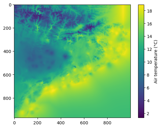
data_field = mlr_id3d_method.interpolate(data)
Now, we can get a quick look of the data_field array using
matplotlib.
import matplotlib.pyplot as plt

plt.imshow(data_field)
plt.colorbar(label='Air temperature (\u00b0C)')
Finally, we can save the result into a GeoTIFF file using
pymica.pymica.PyMica.save_file() from PyMica class.
mlr_id3d_method.save_file("sample-data/results/mlr_id3d.tif")
We have now completed this tutorial on how to interpolate station data
using the mlr methodology combined with residuals correction
(id2d and id3d). You can experiment with changing the
variables_files in the configuration dictionary to observe how the
behavior of each variable affects the interpolation result.